In this chapter we will look at a series of facts about individual or household financial consumption and savings behaviour, examine where that behaviour is inconsistent with traditional economic explanations, and examine possible explanations that can account for the observed behaviour.
Last New Year’s day, after a long evening of rooting the right team to victory in the Orange Bowl, I was lucky enough to win $300 in a college football betting pool. I then turned to the important matter of splurging the proceeds wisely. Would a case of champagne be better than dinner and a play in New York? At this point my son Greg came in and congratulated me. He said, “Gee Dad, you should be pretty happy. With that win you can increase your lifetime consumption by $20 a year!” Greg, it seems, had studied the life-cycle theory of savings.
Despite the economic theory suggesting that people will smooth their incomes over their lifecycle, the observed level of smoothing is low. Consumption responds strongly to both unexpected and predictable changes in income. For example, Broda and Parker (2014) found that the marginal propensity to consume an economic stimulus payment within a quarter is 50-75%. That is, if someone has an unexpected windfall, they will tend to consume 50% to 75% of that windfall within that quarter, rather than saving it.
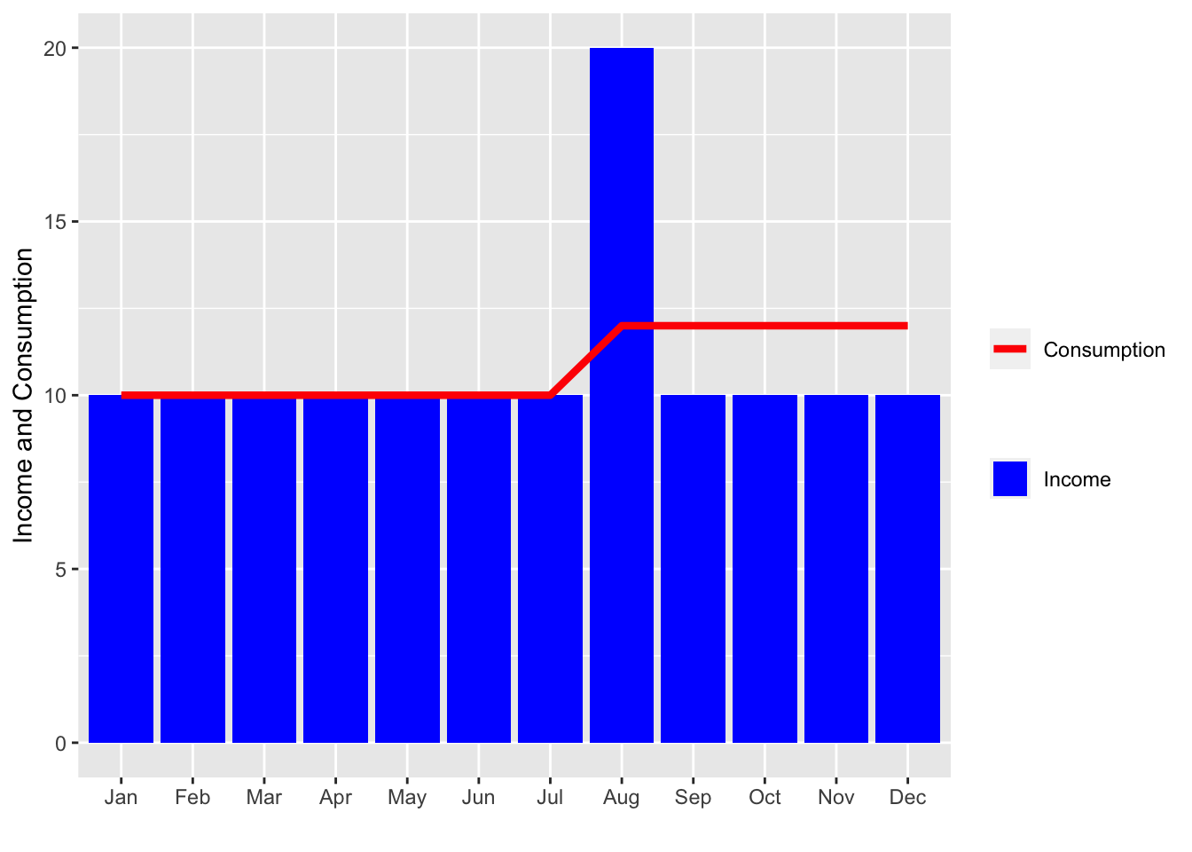
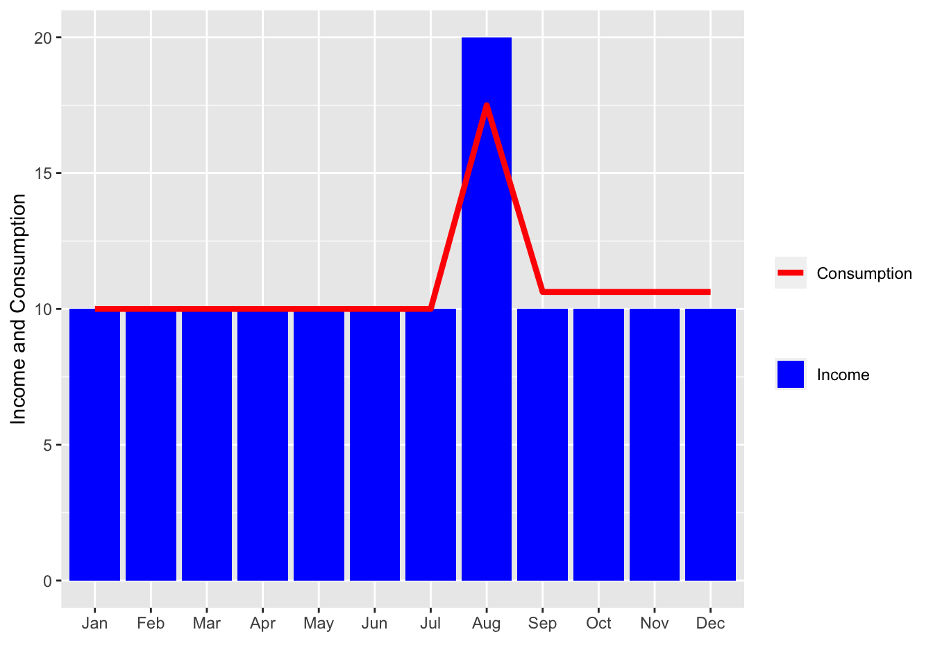
Suppose a patient person anticipates a regular fixed income of $10 a month during their one year of life. In this world there is no inflation or interest paid on borrowing or savings. Further imagine that they received a surprise windfall in August. Someone who perfectly smoothed consumption would spread that surprise over the remaining months of their life.
What we tend to see instead is this - a large spike in consumption at the time of the surprise, with only some of the windfall smoothed over coming months. (In this chart I have assumed that they consume 75% of any income shock when it occurs.)
This lack of smoothing is observed in relation to many major life events. For example, one US study found that when households reach end of unemployment benefits, which in the US have a predictable end date, consumption falls by 13% at that end. Consumption also tends to fall with income at retirement.
The effect of windfalls on our consumption path depends heavily on whether they relate to liquid assets or not. (A liquid asset is one that can readily be converted to cash. Cash is, of course, highly liquid. A house is illiquid as it takes considerable time and effort to convert.) We blow windfall gains of cash, but not windfalls of less liquid assets. For instance, if there is a large increase in share value, we tend not to spend it. But if a company takeover delivers a cash payment, we will tend to spend it rather than smooth consumption of that payment over our lifetime.
12.2 Lifetime savings
In conjunction with this lack of consumption smoothing, households do not tend to accumulate substantial liquid assets over their lifetime. However, they do accumulate substantial illiquid assets.
In Australia, two of the most prominent illiquid assets are housing and superannuation account balances. Liquid assets comprise only around 15% of total household wealth, with less than 2% of that liquid wealth held by the least wealthy half of households (Adams et al. (2020)).
12.3 Rational explanations
There are a number of rational explanations for the lack of observed consumption smoothing. Below are three.
12.3.1 Liquidity constraints
The first relates to liquidity, in that people are unable to sell claims to their future labour income or borrow substantial sums in expectation of its receipt. They cannot simply access the net present value of their lifetime earnings and consume smoothly through time. They have access to less liquidity than the net present value of future earnings.
Consider the increase in lifetime income you could obtain by completing this course. Could you now go to a bank, tell them about this great course you are completing and how it will affect your future income, and then borrow on the basis of that expectation?
As they cannot access future income growth, people increase their consumption as their income grows.
This explanation, however, does not adequately explain the size of the co-movement between income and consumption unless they are highly impatient. But that level of impatience would not accord how much we do accumulate assets. People often accumulate substantial illiquid assets over their life. The explanation does not cover the full range of behaviour that we see.
12.3.2 Dependants
The cost of child rearing often peaks at the same time as earnings (think private school fees). Further, there is little evidence of changes in household consumption as children leave the house, implying that per person consumption increases. This suggests the alignment of child rearing and the peak of earnings may just be coincidence.
12.3.3 Durables
People purchase many “durables” during their lives. These are lumpy purchases that do not quickly wear out and provide utility over time. They are not “consumed” in one use.
Cars and houses are durables. Household goods such as furniture are also durables.
Economists often use expenditure as a proxy for consumption. Durables can make expenditure lumpy (not smoothed) even though the durable good’s consumption occurs over time (is smooth).
There is evidence to support this argument at the micro-level, in that payments such as rent often occur in alignment to pay cycles. On, say, a fortnightly or monthly basis, expenditure does not appear smoothed, whereas consumption is.
However, when we examine the empirical data, durable purchases also do a poor job of explaining the lack of consumption smoothing over a person’s full lifetime.
12.4 Psychological explanations
There are also many explanations for the lack of consumption smoothing based on consumer psychology. Below are three.
12.4.1 Present bias
A prominent explanation of the lack of consumption smoothing is present bias.
Recall from Chapter 6 that present bias (in a quasi-hyperbolic model) involves an immediate discount for any delay at all (\(\beta\)) on top of the regular exponential discount function.
The immediate discount of \(\beta\) generates a distinction between the treatment of liquid and illiquid assets. An illiquid asset is impossible or costly to access for immediate consumption, so any consumption of the illiquid asset is always subject to a delay and a minimum discount of \(\beta\), making is less attractive. Liquid assets such as cash are on hand for consumption now.
Someone with high present bias (i.e. \(\beta\) substantially below one) will have trouble holding any liquid assets, but could accumulate substantial illiquid assets if they do not have a high rate of exponential discounting (i.e. \(\delta\) is close to one).
A related concept is myopia, whereby people consider their income over a limited horizon. This was a feature of Milton Friedman’s (1957) original model of consumption smoothing. If people only think about their income for, say, the next three years, you will see some smoothing. But that smoothing will be limited compared to changes in income and consumption over the complete lifecycle.
12.4.2 Mental accounting
Mental accounting provides a potential explanation for the differences in consumption based on where income came from and what bucket it is currently in. For instance, windfall gains may be in a different mental account to a pay rise, and consumed differently.
One mental account may be for wealth saved for retirement. US data suggests that the medium-term (6-month) marginal propensity to consume out of retirement accounts is effectively zero. The medium marginal propensity to consume out of a transaction account is close to one.
Mental accounts can also be defined around categories of expenditure. For example, money in form of shopping coupons increases shopping more than would be predicted by consumption smoothing. The value of the coupon is not spread over all expenditures.
Mental accounting has some similarity to the liquidity explanation, but in the case of mental accounting it is a self-imposed category or rule. Liquidity constraints are external or natural features of the asset.
12.4.3 Reference point models
Under prospect theory, utility is measured from a reference point. This reference point might be expectations for current consumption, which means that changes in consumption relative to expectations could generate (or cause the loss of) utility.
Suppose today I get to consume five pieces of chocolate. If I had previously expected to consume four pieces, this could generate extra utility. However, if I had previously expected to consume six, this would be painful. In fact, due to loss aversion, it would be more painful than the equivalent pleasant surprise.
This concept can lead to over-consumption, under-savings and high levels of co-movement between income and consumption (if you calibrate the model with certain parameters). For instance, a windfall in income today could be used to markedly increase consumption above expectations, giving a person utility both from the consumption itself and the pleasant surprise. Any consumption shifted into the future would not generate a pleasant surprise on the day of consumption, as by that time it would be expected.
A person’s reference point may also be the consumption of others. Bertrand and Morse (2016) argued that consumption among rich households had induced those at lower income to consume a larger share of their income.
Bertrand, M., and Morse, A. (2016). Trickle-down consumption. Review of Economics and Statistics, 98(5), 863–879. https://doi.org/10.1162/REST_a_00613
Broda, C., and Parker, J. A. (2014). The economic stimulus payments of 2008 and the aggregate demand for consumption. Journal of Monetary Economics, 68, S20–S36. https://doi.org/10.1016/j.jmoneco.2014.09.002
Thaler, R. H. (1990). Anomalies: Saving, fungibility, and mental accounts. Journal of Economic Perspectives, 4(1), 193–205. https://doi.org/10.1257/jep.4.1.193